Topic 7: Inference for the Difference in Means

Difference of Two Means

Motivating Example: A/B testing is a user experience research methodology where two variants of a page are shown to users at random. A company wants to evaluate whether users will spend more time, on average, on page that uses the company’s standard design or on a page with an updated modern design using an A/B test.

Difference of Two Means

The data: To answer this question, the 65 study participants are randomly assigned to view a webpage either using the standard design or the updated design.

• 33 participants viewed the page with the standard design. These participants spent an average of 1.77 minutes on the page, with a standard deviation of 1.68 minutes.

• 32 participants viewed the page with updated design. These participants spent an average of 2.22 minutes on the page, with a standard deviation of 2.09 minutes.

Difference of Two Means

\[\overline{x}_S = 1.77 \text{ min}\] \[ s_S = 1.68 \text{ min}\] \[n_S = 33\]  

\[\overline{x}_U = 2.22 \text{ min}\] \[s_U = 2.09 \text{ min}\] \[n_U = 32\]

Estimation

A Confidence Interval for the Difference in Means, \(\mu_1-\mu_2\)

1. Calculate the point estimate, \(\overline{x}_1 - \overline{x}_2\)

2. Identify the confidence level, \(CL\), and the error associated with this confidence level \(100-CL\).

3. Determine the critical value, \(t^*\), by finding the \(CL + \frac{100-CL}{2}\) percentile on the t distribution with \(\nu\) degrees of freedom (df).

   • \(\nu\) represents the Satterthwaite degrees of freedom (see next slide)

4. Calculate the standard error estimate from the observed sample:

\[\sqrt{\frac{s_1^2}{n_1}+\frac{s_2^2}{n_2}}\]

Sattherthwaite Degrees of Freedom, \(\nu\)

Link to this calculator and an R script alternative is available in the Week 8 Canvas module.

Finding t Critical Values using qt()

 

qt(p, df) calculates the value on a t distribution curve with df degrees of freedom that has an area of p to the left of it.

 

Example: To find the critical value needed to construct a 99% confidence interval for the difference in means when \(s_1 = 1.68\), \(n_1 = 33\), \(s_2 = 1.09\), \(n_2 = 32\):

qt(0.995, 59.419)

[1] 2.661134

Confidence Interval Construction for \(\mu_1-\mu_2\)

 

(\(\overline{x}_1 - \overline{x}_2)\) \(\pm\) \(t^*_{\nu}\) \(\sqrt{\frac{s_1^2}{n_1}+\frac{s_2^2}{n_2}}\)

 

Motivating Example: Construct the 99% confidence interval for the difference in the mean time spent on the Standard Site and the Updated Site.

(\(1.77-2.22)\) \(\pm\) \(2.661\) \(\sqrt{\frac{1.68^2}{33}+\frac{2.09^2}{32}}\)

(1.77 - 2.22) + c(-1,1)*qt(0.995, 59.419)*sqrt(((1.68^2)/33) + ((2.09^2)/32))

[1] -1.7039291  0.8039291

 

Practice! 🐓

 

 

Answer questions 1-6 on the Class 15 Activity - Difference in Means activity on Canvas.

 

Leave the activity open. We’ll come back to it.

07:00

Hypothesis Testing

Testing for a Difference in Means

• We can perform a formal hypothesis test to answer questions concerning a difference in two population means.

• We’ll use the same steps introduced in our Introduction to Hypothesis Testing notes, but some of the details will differ in this new scenario.

1. Identify the question and parameter of interest.

 

Motivating Example:

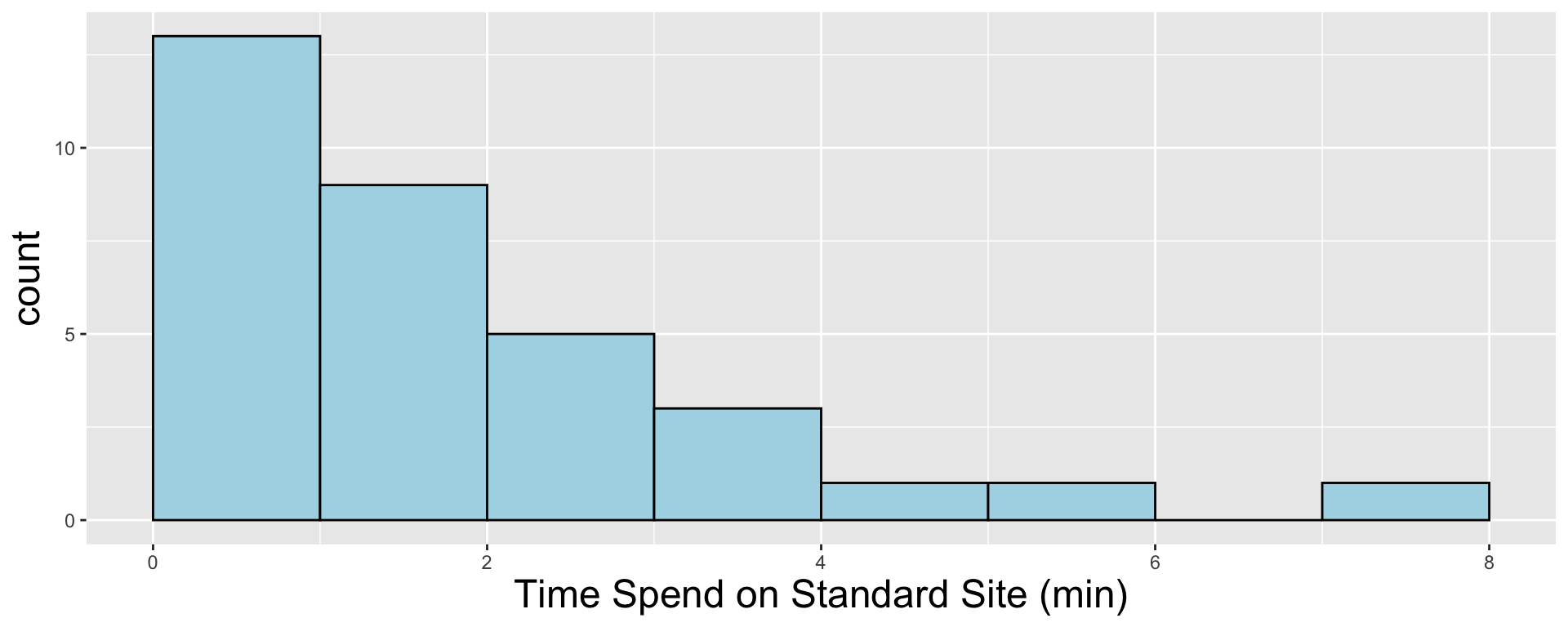
Is there a difference in the average amount of time users spend on the Standard Site vs. the Updated Site?

 

The parameter of interest:

The difference in the average amount of time spent on the two sites, \(\mu_S - \mu_U\)

2. Set up the null and alternative hypotheses

Null hypothesis

\[H_0: \mu_1 = \mu_2\]

Alternative hypothesis:

This depends on the question of interest.

Lower one-sided

Question of interest: Is the mean of population 1 less than the mean of population 2?

\(H_A: \mu_1 <\mu_2\)

Upper one-sided

Question of interest: Is the mean of population 1 greater than the mean of population 2?

\(H_A: \mu_1 >\mu_2\)

Two-sided

Question of interest: Is the mean of population 1 different from the mean of population 2?

\(H_A: \mu_1 \neq\mu_2\)

2. Set up the null and alternative hypotheses

 

Motivating Example:

 

\(H_0:\)\(\mu_S = \mu_U\)

 

\(H_A:\mu_S \neq \mu_U\)

Practice! 🐓

 

 

Answer questions 7-8 on the Class 15 Activity - Difference in Means activity on Canvas.

 

Leave the activity open. We’ll come back to it.

02:00

3. Collect and summarize the data.

Motivating Example:

\[\overline{x}_S = 1.77 \text{ min}\] \[ s_S = 1.68 \text{ min}\] \[n_S = 33\]

 

 

\[\overline{x}_U = 2.22 \text{ min}\] \[s_U = 2.09 \text{ min}\] \[n_U = 32\]

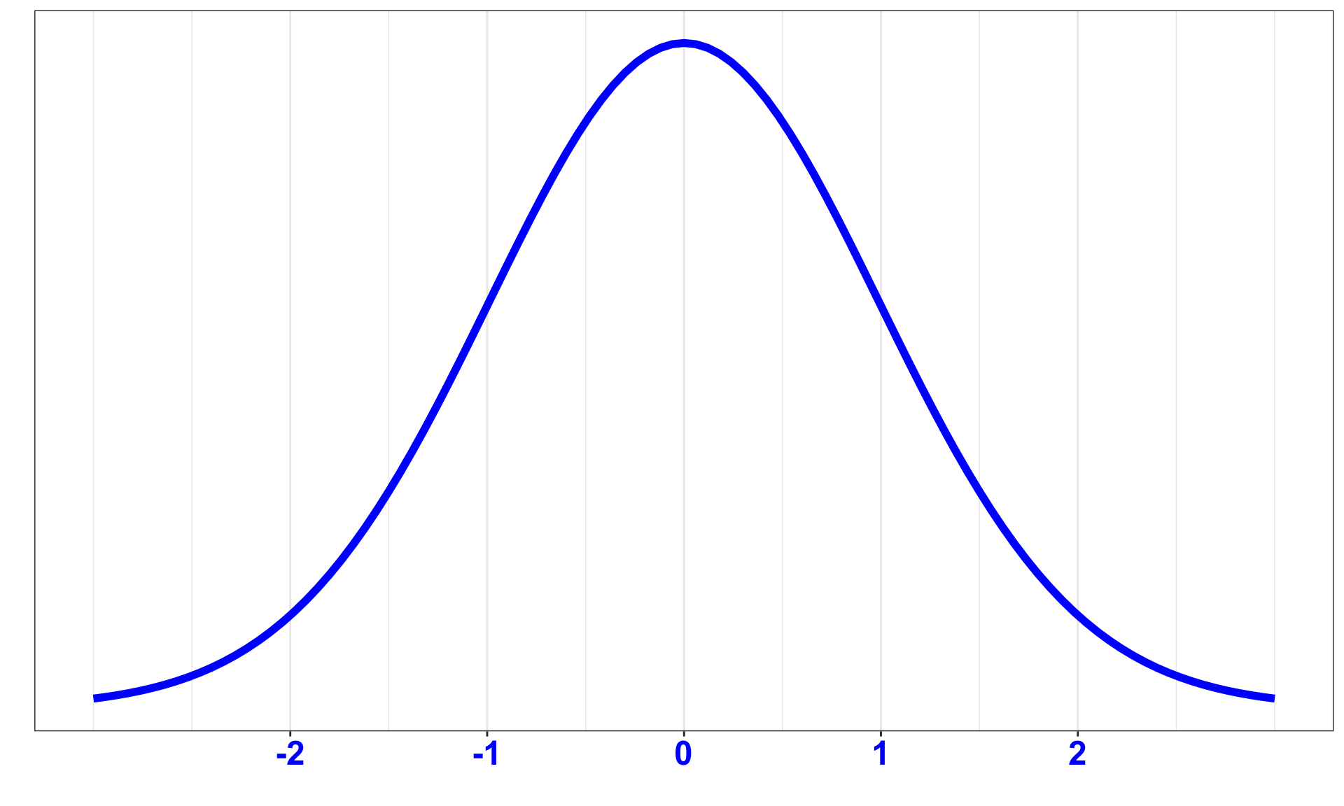
4. Determine the Null Distribution

 

If the sample sizes are sufficiently large, under the null hypothesis, the distribution of the test statistic used in testing the difference between two population means is a

t distribution with \(\nu\) degrees of freedom.

\(\nu\) represents the Satterthwaite degrees of freedom.

 

How large do the samples need to be?

• If both \(n_1\geq 30\) and \(n_2 \geq 30\), we can move forward.

• If either \(n_1 < 30\) or \(n_2 < 30\), we need to look at the sampled distribution(s) of the small sample(s). If there are no clear outliers or strong skewness in the sampled data, we can move forward. If either sampled distribution suggests skewness or outliers, we should not proceed.

4. Determine the Null Distribution

Motivating Example:

Are the sample sizes sufficiently large?

Yes, both \(n_1\geq\) and \(n_2\geq30\).

 

So the null distribution is at distribution with 59.419 degrees of freedom.

5. Calculate the test statistic

When testing the difference in population means, \(\mu_1\) vs. \(\mu_2\), the test statistic is

 

\[t = \frac{\overline{x}_1-\overline{x}_2}{\sqrt{\frac{s_1^2}{n_1} + \frac{s_2^2}{n_2}}}\]

 

5. Calculate the test statistic

When testing the difference in population means, \(\mu_1\) vs. \(\mu_2\), the test statistic is

 

\[t = \frac{\overline{x}_1-\overline{x}_2}{\sqrt{\frac{s_1^2}{n_1} + \frac{s_2^2}{n_2}}}\]

 

Motivating Example:

\[t = \frac{1.77-2.22}{\sqrt{\frac{1.68^2}{33} + \frac{2.09^2}{32}}} = -0.955\]

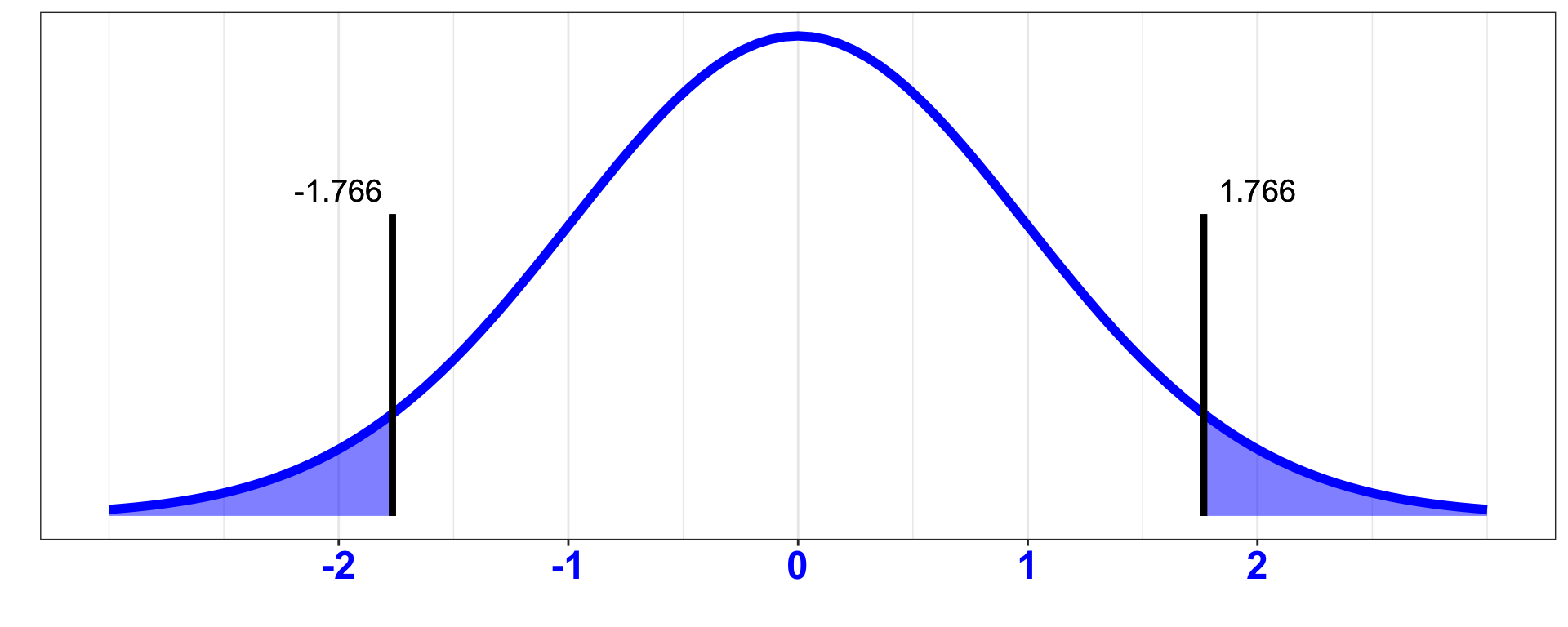
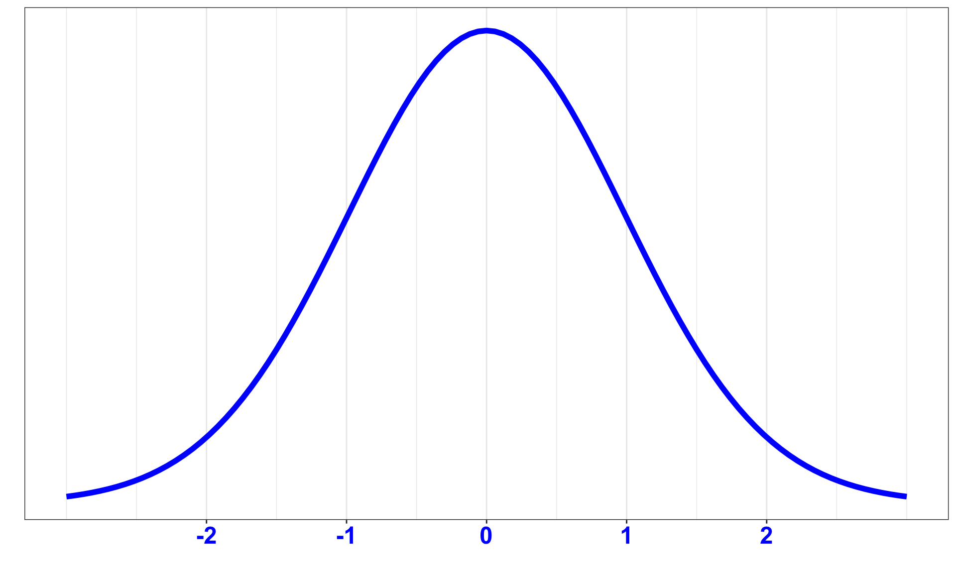
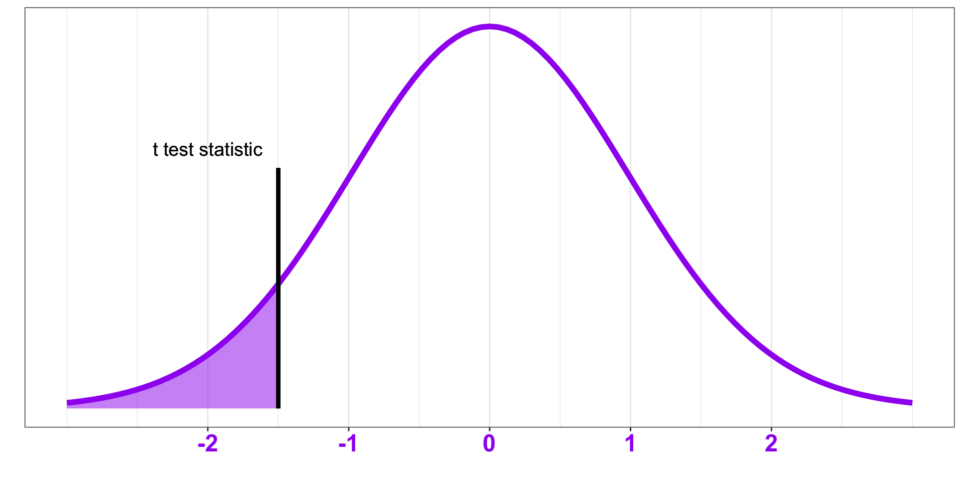
6. Calculate the p-value using the test statistic and null distribution.

Lower one-sided:

\(H_A: \mu_1<\mu_2\)

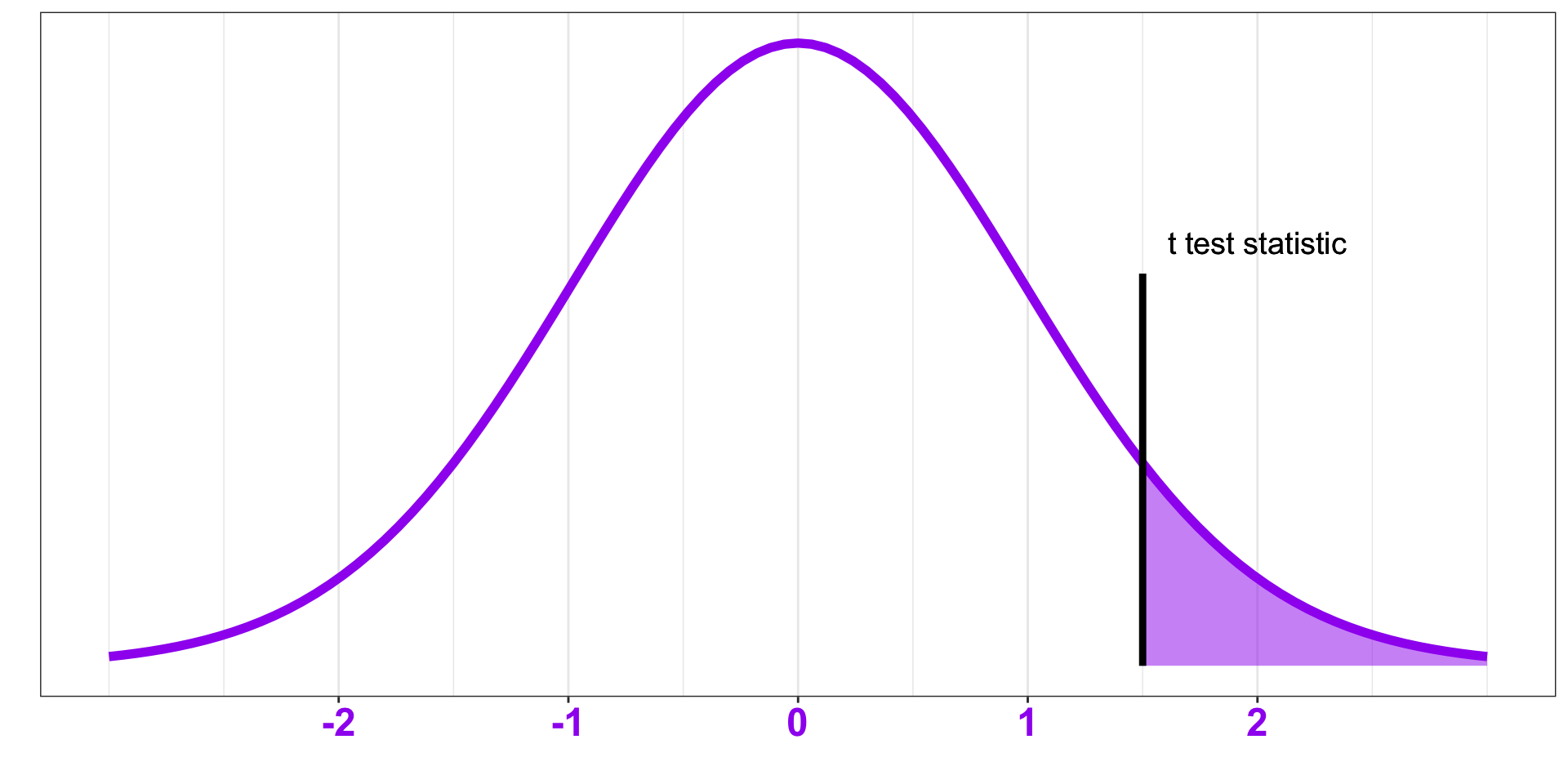
Upper one-sided:

\(H_A: \mu_1>\mu_2\)

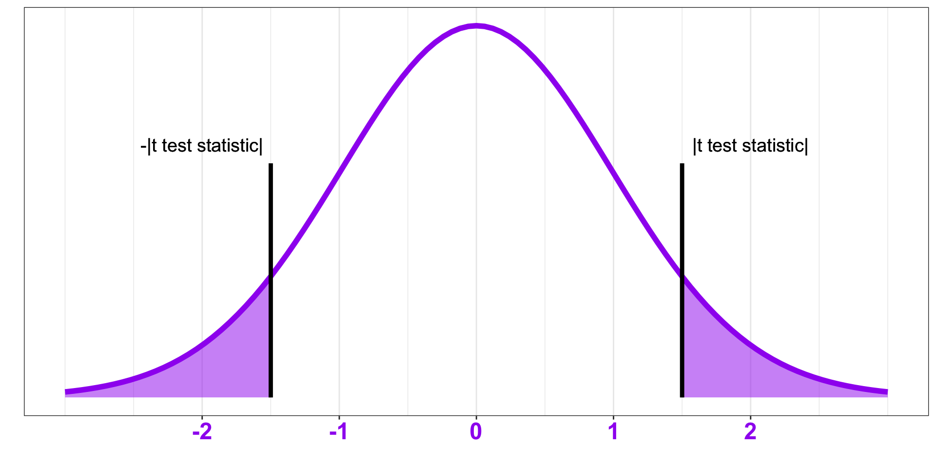
Two-sided:

\(H_A: \mu_1\neq \mu_2\)

R code:

pt(t, df)

R code:

1-pt(t, df))

R code:

2*(1-pt(abs(t), df))

where df is the Satterthwaite degrees of freedom, \(\nu\)

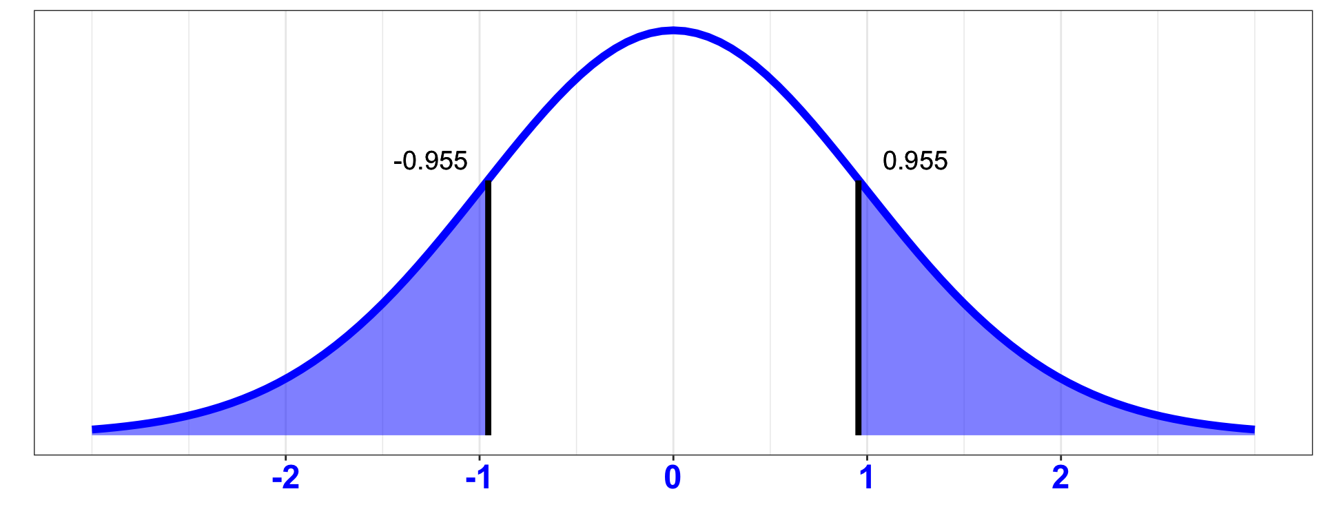
6. Calculate the p-value using the test statistic and null distribution.

Motivating Example:

 

2*(1-pt(abs(-0.955), 59.419)) = 0.343

Practice! 🐓

 

 

Answer questions 9-11 on the Class 15 Activity - Difference in Means activity on Canvas.

02:00

7. Make a conclusion

Write a 4-part conclusion. The conclusion should be written in the context of the problem and contain the following components:

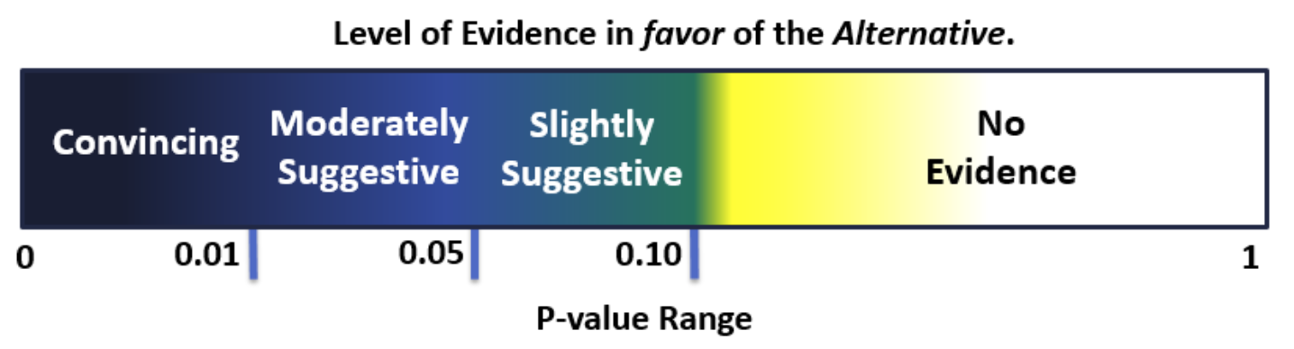
1. A statement for the strength of evidence in favor the alternative hypothesis.

2. Whether to reject or fail to reject the null hypothesis.

3. The point estimate for the parameter of interest.

4. A \((1-\alpha)100\%\) confidence interval estimate for the parameter of interest.

7. Make a conclusion

A statement in terms of the alternative hypothesis

• Using terms like “reject” and “fail to reject the null” may be confusing to novice readers.
• We’ll provide a more complete conclusion by providing a statement of evidence in terms of the alternative hypothesis that reflects the question of interest.

7. Make a conclusion

Motivating Example: Write a 4-part conclusion with a \(\alpha=0.01\) significance level.

1. There is no evidence that the mean time spent on the Standard Site differs from the mean time spent on the Updated Site.

2. At the \(\alpha=0.01\) significance level, we fail to reject the null hypothesis.

3. and 4. We are 99% confident that the users spend 1.70 minutes less to 0.80 minutes more on the Standard Site than on the Updated Site, on average, with an estimated difference of 0.45 more minutes spent on the Updated Site on average.