Topic 10 - Inference for Linear Regression

Download or print notes to PDF

If you’d like to export this presentation to a PDF, do the following

Toggle into Print View using the E key.
Open the in-browser print dialog (CTRL/CMD+P)
Change the Destination to Save as PDF.
Change the Layout to Landscape.
Change the Margins to None.
Enable the Background graphics option.
Click Save.

This feature has been confirmed to work in Google Chrome and Firefox.

Inference for Linear Regression

Recall that if we’re using a sample of data to try and model the true relationship between two quantitative variables, then the intercept, $b_0$, and slope, $b_1$, estimates are random variables.

$\hat{y} = 1994.39 + 46.68 x$

$\hat{y} = 1191.82 + 62.98 x$

Estimating Parameters

The LSRL is based on sampled data, so \[\hat{y} = b_0 + b_1x\] is the estimate for the true population regression equation \[y = \beta_0 + \beta_1 x + \varepsilon\]

$b_0$ is the point estimate for $\beta_0$
$b_1$ is the point estimate for $\beta_1$
$\varepsilon$ is the error (variability around the regression line)

Our focus from here on out will be on inference about the slope parameter, $\beta_1$.

Inference about $\beta_1$

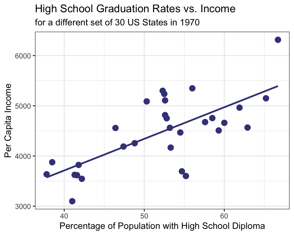
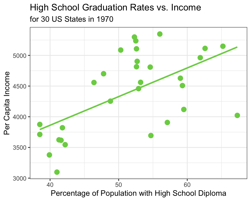
Consider the LSRL for the relationship between the percentage a state’s population with a high school diploma and per capita income.

$\hat{y} = 1994.39 + 46.68 x$

The slope in the LSRL, $46.68$, is an estimate for the true population regression line.

We might wonder, do these data provide strong evidence that the percentage of HS graduates is useful predictor of a state’s per capita income?

Frame this question of interest into a hypothesis test:

$H_0:$ $\beta_1 = 0$ The true linear model has slope zero.

$H_A:$ $\beta_1 \neq 0$ The true linear model has a slope different than zero. The explanatory variable is good predictor of the response.

Using Software Output to Perform a Hypothesis Test on $\beta_1$

R Code:

LSRL <- lm(Income ~ HSGrad, data = state_30)
summary(LSRL)


Call:
lm(formula = Income ~ HSGrad, data = state_30)

Residuals:
     Min       1Q   Median       3Q      Max 
-1113.99  -314.05    36.65   389.53   863.22 

Coefficients:
            Estimate Std. Error t value Pr(>|t|)    
(Intercept)  1994.39     634.62   3.143 0.003935 ** 
HSGrad         46.68      12.18   3.832 0.000658 ***
---
Signif. codes:  0 '***' 0.001 '**' 0.01 '*' 0.05 '.' 0.1 ' ' 1

Residual standard error: 537.3 on 28 degrees of freedom
Multiple R-squared:  0.344, Adjusted R-squared:  0.3206 
F-statistic: 14.68 on 1 and 28 DF,  p-value: 0.0006581

Interpreting the p-value and drawing a conclusion

Perform a hypothesis test on the slope parameter, $\beta_1$, using a significance level of $\alpha = 0.05$.

The p-value for the hypothesis test on the slope parameter is $0.000658$.

Since $0.000658 < \alpha$, we will reject the null hypothesis.

There is convincing evidence that the percentage of high school graduates is a useful predictor of a state’s per capita income in the 1970s.

Confidence Interval Estimates for $\beta_1$

In addition to performing a hypothesis test about the slope parameter, we can provide a measure of uncertainty about the estimate for $\beta_1$ by constructing a confidence interval for the parameter.

\[b_1 \pm t^* \times SE_{b_1}\]

The standardized estimate for $\beta_1$, $\frac{b_1}{SE_{b_1}}$, follows a t-distribution with $n-2$ degrees of freedom. We will use this distribution to determine $t^*$.

qt(p, df)

where p corresponds to the area under the t-distribution curve to the left of the critical value and df $n-2$.

Confidence Interval Estimate for $\beta_1$

Construct the 95% confidence interval for the slope parameter of high school graduation rate on life expectancy.

For $b_1$ and $SE_{b_1}$, use the model output in R:

              Estimate Std. Error  t value     Pr(>|t|)
(Intercept) 1994.38858  634.62049 3.142648 0.0039352579
HSGrad        46.68049   12.18172 3.832013 0.0006580844

Calculate the critical value, $t^*$:

qt(0.975, 28)

[1] 2.048407

Compute the lower and upper bounds of the interval:

46.68049 + c(-1,1)*qt(0.975, 28)*12.18172

[1] 21.72737 71.63361

We are 95% confident that for each additional percentage of the population with a high school diploma, per capita income is expected to increase by $21.72 to $71.63, with a point estimate for the increase of $46.68.

R Code for This Week’s Examples

# Open the tidyverse library
library(tidyverse)

# Import the dataset, first need to download the data from Canvas
state_30 <- read_csv(file.choose())

# Create a scatterplot of the Illiteracy and LifeExp variables
state_30 |>
  ggplot(aes(x = `HS Grad`, y = Income)) +
  geom_point(color = viridis::viridis(6)[5], size = 3) + 
  labs(y = "Per Capita Income", 
       x = "Percentage of Population with High School Diploma", 
       title = "High School Graduation Rates vs. Income ",
       subtitle = "for 30 US States in 1970") + 
  theme(axis.title = element_text(size = 18)) + 
  theme_bw() + 
  stat_smooth(method = "lm",
              formula = y ~ x, 
              geom = "smooth", 
              se = FALSE, 
              color = viridis::viridis(6)[5])

# Rename HS Grad variable
state_30 <- state_30 |>
  rename("HSGrad"=`HS Grad`)

# Estimate intercept and slope for LSRL
LSRL <- lm(Income ~ HSGrad, data = state_30)
summary(LSRL)

Practice

Please complete the Class 19 Activity - SLR in Canvas.

Topic 10 - Inference for Linear Regression

Download or print notes to PDF

Inference for Linear Regression

Estimating Parameters

Inference about \(\beta_1\)

Using Software Output to Perform a Hypothesis Test on \(\beta_1\)

Interpreting the p-value and drawing a conclusion

Confidence Interval Estimates for \(\beta_1\)

Confidence Interval Estimate for \(\beta_1\)

R Code for This Week’s Examples

Practice